机械臂的动力学部分

5.1 机械臂动力学的目标#

机械臂动力学的目标是在已知机械臂模型（关节设置）和各个连杆和质量分布的情况下，给定机械臂末端期望实现的位姿、速度、加速度，求在各个关节的制动器上应该施加的力或力矩。

5.2 迭代法求解动力学问题#

5.2.1 符号约定#

对于连杆 $i$ ，有三个与之相关联的框架，分别是

连杆 $i$ 的在关节轴 $i$ 处的固连框架 $\{i\}$
在连杆 $i$ 的质心 $c_i$ 处的质心固连框架 $\{c_i\}$ ，其朝向与框架 $\{i\}$ 一致
在关节轴 $i+1$ 处的连杆 $i+1$ 的固连框架 $\{i+1\}$

约定连杆 $i$ 的质量为 $m_i$ ，相对于质心框架 $\{c_i\}$ 的惯性张量为 $^{c_i}I_i$ ; 相对于刚体自身框架，关节 $i$ 处的线速度和线加速度为 $^{i}v_i, \ ^{i}\dot v_i$ ，连杆 $i$ 的角速度及角加速度为 $^{i}\omega_i, \ ^{i}\dot \omega$ ，连杆 $i - 1$ 施加在连杆 $i$ 上的力和力矩为 $^{i}f_i, \ ^{i}n_i$ ，连杆 $i$ 施加在连杆 $i+1$ 上的力和力矩为 $^{i}f_{i+1},\ ^{i} n_{i+1}$

5.2.2 牛顿-欧拉动力学方程#

对于连杆 $i$ ，有

\begin{aligned} \vec{f}_i - \vec{f}_{i+1} + m_i \vec{g} &= m_i \dot{\vec{v}}_{c_i} \\ ^{c_i}\left[\vec{n}_i - \vec{n}_{i+1} + (\vec{p}_i - \vec{p}_{c_i}) \times \vec{f}_i - (\vec{p}_{i+1} - \vec{p}_{c_i} \times \vec{f}_{i+1})\right] &= \ ^{c_i}I_{c_i}\ ^{c_i} \dot\omega_{c_i} + \ ^{c_i}\omega_{c_i} \times \ ^{c_i}I_{c_i}\ ^{c_i}\omega_{c_i} \end{aligned}

其中 $^{c_i}[\cdot]$ 表示将物理矢量表达成框架 $\{c_i\}$ 中的数学向量。

由方程可知，为了求解 $f_i$ 与 $f_{i+1}$ ，需要先求出 $\dot{\vec{v}}_{c_i}$ 、 $\vec{\omega}_{c_i}$ 和 $\dot{\vec{\omega}}_{c_i}$

5.2.3 前向迭代求速度#

线加速度

按照上一章的速度传播结果，可以先求出关节 $i$ 处的速度 $v_i$ ，然后，求出连杆 $i$ 质心处的速度 $v_{c_i}$ 。注意质心框架 $\{c_i\}$ 与框架 $\{i\}$ 的朝向一致，

\begin{aligned} ^{c_i} v_{c_i} &= \ ^{i}v_{c_i} = \ ^{i}v_i + \ ^{i}\omega_i \times \ ^{i}p_{c_i} \end{aligned}

其中， $^{i}p_{c_i}$ 表示质心 $c_i$ 在框架 $\{i\}$ 中的位矢的向量表达。直接对时间 $t$ 求导，可以得到线加速度为

^{c_i} \dot{v}_{c_i} = \ ^{i}\dot{v}_{c_i} = \ ^{i}\dot{v}_i + \ ^{i}\dot{\omega}_i \times \ ^{i}p_{c_i} + \ ^{i}{\omega}_i \times (\ ^{i}{\omega}_i \times \ ^{i}p_{c_i})

其中最后一项是对 $^{i}p_{c_i}$ 求导的结果，这里是由于朝向发生了变化因此有一项导数。

角速度及角加速度

由于

\begin{aligned} ^{c_i} \omega_{c_i} = \ ^{i}\omega_{c_i} = \ ^{i}\omega_i \end{aligned}

有

^{c_i} \dot\omega_{c_i} = \ ^{i}\dot\omega_{c_i} = \ ^{i}\dot\omega_i

5.2.4 反向迭代求动力#

对于连杆 $i$ ，假设此时 $^{i+1}f_{i+1}$ 和 $^{i+1}n_{i+1}$ ，有

\begin{aligned} ^{i}F_i & = m_i \ ^{c_i}\dot v_{c_i}\quad \text{惯性力， 作用于质心} c_i\\ ^{i}N_i & = \ ^{c_i}I \ ^{i} \dot \omega_{i} + \ ^{i}\omega_i \times \ ^{c_i}I \ ^{i}\omega_i \quad \text{惯性力矩}\\ ^{i}f_i &=\ ^{i}F_i + \ ^{i}_{i+1}R \ ^{i+1}f_{i+1} - m_i\ ^{i}g \quad \text{牛顿第二定律}\\ ^{i}n_i &=\ ^{i}N_i + \underbrace{\ ^{i}p_{c_i} \times \ ^{i}F_i}_{N_i\text{的平移附加项}} + \ ^{i}_{i+1}R \ ^{i+1}n_{i+1} + \underbrace{\ ^{i}p_{i+1} \times \ ^{i}_{i+1}R \ ^{i+1}f_{i+1}}_{n_{i+1}\text{的平移附加项}} - \ ^{i}p_{c_i} \times m_i \ ^{i}g \quad\text{相对于关节}i\text{处的力矩方程} \end{aligned}

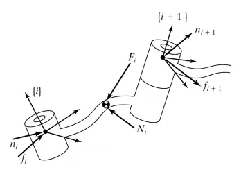
注意这里的重力项 $m_i\ ^{i}g$ 和 $\ ^{i}p_{c_i} \times m_i \ ^{i}g$ 需要依据问题环境来设置，有时候可以不用考虑重力项
注意重力项是被减去的！(例如，设置 $^{0}g = \begin{bmatrix} 0 \\ -|g| \\ 0\end{bmatrix}$ )
有时候还需要考虑粘滞阻力等其他外力，此时需要对方程做相应修改。

迭代的初始条件通常是机械臂末端是自由运动的，即

\begin{aligned} ^{N+1}f_{N+1} &= 0\\ ^{N+1}n_{N+1} &= 0 \end{aligned}

这里 $N$ 是关节个数，设置为大写是为了与力矩向量 $n$ 区分。

5.2.5 关节提供的动力#

关节只负责提供 Z 轴方向的动力，于是可以求出

棱柱关节需要提供的力 $\tau_i = \ ^{i}f_i ^\top \ ^{i}\mathbf{\hat{z}}_i$
旋转关节需提供的力矩 $\tau_i = \ ^{i}n_i ^\top \ ^{i}\mathbf{\hat{z}}_i$

5.2.6 特别需要注意的地方#

特别需要注意，这里面对速度 $v$ 和 $\omega$ 是不可以直接对向量表达求导的，这样得到的结果是错误的！！！ 具体的原因是在整个运动的过程中，框架也是在发生变化的，对应于物理学中矢量的求导是需要分矢量的标量大小和矢量方向求导两个部分的。下面的例题将说明这一点。

(角速度部分的 $\dot\theta$ 由于是对标量求导，所以不会存在这个问题)

平面2R的动力学模型

简化质量分布，假设每个连杆的质量都集中在连杆远端的一点，分别是 $m_1$ 和 $m_2$ ，重力沿着 $\{0\}$ 框架 Y 轴负方向。

解：

前向运动学方程为

\begin{aligned} ^{0}_{1}T &= \begin{bmatrix} c\theta_1 & -s\theta_1 & 0 & 0\\ s\theta_1 & c\theta_1 &0 &0\\ 0 &0 &1 &0 \\ 0 &0 &0 &1\end{bmatrix} \\ ^{1}_{2}T &= \begin{bmatrix} c\theta_2 & -s\theta_2 & 0 & L_1\\ s\theta_2 & c\theta_2 &0 &0\\ 0 &0 &1 &0 \\ 0 &0 &0 &1\end{bmatrix} \\ ^{2}_{3}T &= \begin{bmatrix} 1 & 0 & 0 & L_2\\ 0 & 1 &0 &0\\ 0 &0 &1 &0 \\ 0 &0 &0 &1\end{bmatrix} \\ ^{0}_{3}T(\theta_1, \theta_2) &= \begin{bmatrix} c(\theta_1 + \theta_2) & -s(\theta_1 + \theta_2) & 0 & L_1 c\theta_1 + L_2 c(\theta_1 + \theta_2)\\ s(\theta_1 + \theta_2) & c(\theta_1 + \theta_2) &0 &L_1 s\theta_1 + L_2 s(\theta_1 + \theta_2)\\ 0 &0 &1 &0 \\ 0 &0 &0 &1\end{bmatrix} \\ \end{aligned}

前向速度传播的结果为 (初始条件 $^0\omega_0 = 0, \ ^0v_0 = 0$ )，利用迭代公式，有

\begin{aligned} \ ^{1}\omega_1 &= \ ^{1}_{0}R \ ^{0}w_0 + \dot\theta_1 \ ^{1}\mathbf{\hat{z}}_1 = \begin{bmatrix}0\\ 0\\ \dot\theta_1\end{bmatrix}\\ \ ^{2}\omega_2 &= \ ^{2}_{1}R \ ^{1}w_1 + \dot\theta_2 \ ^{2}\mathbf{\hat{z}}_2 = \begin{bmatrix} 0 \\ 0\\ \dot\theta_1 + \dot\theta_2\end{bmatrix} \\ \\ \ ^{1}v_1 &= \ ^{1}_{0}R(\ ^{0}v_0 + \ ^{0}\omega_0 \times \ ^{0} p_1) = 0\\ \ ^{2}v_2 &= \ ^{2}_{1}R(\ ^{1}v_1 + \ ^{1}\omega_1 \times \ ^{1}p_2) = \begin{bmatrix} L_1\dot\theta_1 s\theta_2 \\ L_1\dot\theta_1c\theta_2 \\ 0\end{bmatrix} \\ ^{1}v_{c_1} &= \ ^{1}v_1 + \ ^{1}\omega_1 \times \ ^{1}p_{c_1} = \begin{bmatrix} 0\\0\\\dot\theta_1\end{bmatrix} \times \begin{bmatrix} L_1 \\0\\0\end{bmatrix} = \begin{bmatrix} 0 \\ L_1\dot\theta_1 \\0\end{bmatrix} \\ ^{2}v_{c_2} &= \ ^{2}v_2 + \ ^{2}\omega_2 \times \ ^{2}p_{c_2} = \begin{bmatrix} L_1\dot\theta_1 s\theta_2 \\ L_1\dot\theta_1c\theta_2 \\ 0\end{bmatrix} + \begin{bmatrix}0 \\0\\ \dot\theta_1 + \dot\theta_2\end{bmatrix} \times \begin{bmatrix} L_2 \\0\\0\end{bmatrix} = \begin{bmatrix} L_1\dot\theta_1 s\theta_2 \\ L_1\dot\theta_1c\theta_2 + L_2 (\dot\theta_1 + \dot\theta_2) \\ 0\end{bmatrix} \end{aligned}

求导，有

\begin{aligned} \ ^{1}\dot\omega_1 &= \ ^{1}_{0}R \ ^{0}\dot \omega_0 + \ ^{1}_{0}R \ ^{0}\omega_0 \times \dot\theta_1 \ ^{1}\mathbf{\hat{z}}_1 + \ddot\theta_1 \ ^{1}\mathbf{\hat{z}}_1 = \begin{bmatrix} 0 \\ 0\\ \ddot\theta_1\end{bmatrix} \\ \ ^{2}\dot\omega_2 &= \ ^{2}_{1}R \ ^{1}\dot\omega_1 + \ ^{2}_{1}R \ ^{1}\omega_1\times \dot\theta_2 \ ^{2}\mathbf{\hat{z}}_2 + \ddot\theta_2 \ ^{2}\mathbf{\hat{z}}_2 = \begin{bmatrix} 0 \\ 0\\ \ddot\theta_1 + \ddot\theta_2\end{bmatrix} \\ \ ^{1}\dot v_1 &= \ ^{1}_{0}R(\ ^{0}\dot\omega_0 \times \ ^{0}p_1 + \ ^{0}\omega_0 \times (\ ^{0}\omega_0 \times \ ^{0}p_1) + \ ^{0}\dot v_0) = 0 \\ \ ^{1}\dot v_{c_1} &= \ ^{1}\dot\omega_1 \times \ ^{1}p_{c_1} + \ ^{1}\omega_1 \times (\ ^{1}\omega_1 \times \ ^{1}p_{c_1}) + \ ^{1}\dot v_{1} = \begin{bmatrix} -L_1\dot\theta_1^2 \\ L_1\ddot\theta_1\\0 \end{bmatrix} \\ \ ^{2}\dot v_2 &= \ ^{2}_{1}R(\ ^{1}\dot\omega_1 \times \ ^{1}p_2 + \ ^{1}\omega_1 \times (\ ^{1}\omega_1 \times \ ^{1}p_2) + \ ^{1}\dot v_1) = \begin{bmatrix} L_1\ddot\theta_1s\theta_2 - L_1\dot\theta_1^2c\theta_2 \\ L_1\ddot\theta_1c\theta_2 + L_1\dot\theta_1^2s\theta_2 \\ 0\end{bmatrix} \\ \ ^{2}\dot v_{c_2} &= \ ^{2}\dot\omega_2 \times \ ^{2}p_{c_2} + \ ^{2}\omega_2 \times (\ ^{2}\omega_2 \times \ ^{2}p_{c_2}) + \ ^{2}\dot v_{2} = \begin{bmatrix}-L_2(\dot\theta_1 + \dot\theta_2)^2 + L_1\ddot\theta_1s\theta_2 - L_1\dot\theta_1^2c\theta_2 \\ L_2(\ddot\theta_1 + \ddot\theta_2) + L_1\ddot\theta_1c\theta_2 + L_1\dot\theta_1^2s\theta_2 \\ 0 \end{bmatrix} \\ \end{aligned}

注意到一个规律可以方便记忆公式，就是如果有矢量 $a = \begin{bmatrix} a_x \\ a_y \\ a_z\end{bmatrix}$ 是在变化的框架中表达的，那么对这个向量求导时，除了有自身在当前框架的直接导数 $\begin{bmatrix} \dot a_x \\ \dot a_y \\ \dot a_z\end{bmatrix}$ 外，还会有框架变化导致的导数 $\omega \times \begin{bmatrix} a_x \\ a_y \\a_z\end{bmatrix}$ 。这个规律适用于上面 $\dot\theta_2 \ ^{2}\mathbf{\hat{z}}_2$ 的导数计算和 $\ ^{1}\omega_1 \times \ ^{1} p_{c_1}$ 的导数计算（这里面 $\ ^{1}\omega_1$ 的大小和框架变化的导数全含在了 $\ ^{1}\dot \omega_1$ 中， $\ ^{1}p_{c_1}$ 没有大小的变化，因此只有框架变化的导数 $(\omega \times p)$ ）。

于是计算惯性力及惯性力矩

\begin{aligned} ^{1}F_1 &= m_1 \ ^{1}\dot v_{c_1} = \begin{bmatrix} -m_1L_1\dot\theta_1^2 \\ m_1L_1\ddot\theta_1\\0 \end{bmatrix} \\ \ ^{2}F_2 &= m_2 \ ^{2}\dot v_{c_2} = \begin{bmatrix}-m_2L_2(\dot\theta_1 + \dot\theta_2)^2 + m_2L_1\ddot\theta_1s\theta_2 - m_2L_1\dot\theta_1^2c\theta_2 \\ m_2L_2(\ddot\theta_1 + \ddot\theta_2) + m_2L_1\ddot\theta_1c\theta_2 + m_2L_1\dot\theta_1^2s\theta_2 \\ 0 \end{bmatrix} \\ \ ^{1}N_1 &= \ ^{c_1}I \ ^{1} \dot \omega_{1} + \ ^{1}\omega_1 \times \ ^{c_1}I \ ^{1}\omega_1 = 0 \\ \ ^{2}N_2 &= \ ^{c_2}I \ ^{2} \dot \omega_{2} + \ ^{2}\omega_2 \times \ ^{c_2}I \ ^{2}\omega_2 = 0 \end{aligned}

带入公式，结合 $\ ^{3} f_3 = 0, \ ^{3} n_3 = 0$ 得

\begin{aligned} \ ^{2}f_2 &= \ ^{2}F_2 + \ ^{2}_{3}R \ ^{3}f_{3} - m_2\ ^{2}g = \begin{bmatrix}-m_2L_2(\dot\theta_1 + \dot\theta_2)^2 + m_2L_1\ddot\theta_1s\theta_2 - m_2L_1\dot\theta_1^2c\theta_2 \\ m_2L_2(\ddot\theta_1 + \ddot\theta_2) + m_2L_1\ddot\theta_1c\theta_2 + m_2L_1\dot\theta_1^2s\theta_2 \\ 0 \end{bmatrix} - m_2 \ ^{2}_{0}R\begin{bmatrix} 0 \\ -g \\ 0\end{bmatrix} = \begin{bmatrix}-m_2L_2(\dot\theta_1 + \dot\theta_2)^2 + m_2L_1\ddot\theta_1s\theta_2 - m_2L_1\dot\theta_1^2c\theta_2 + m_2gs(\theta_1 + \theta_2) \\ m_2L_2(\ddot\theta_1 + \ddot\theta_2) + m_2L_1\ddot\theta_1c\theta_2 + m_2L_1\dot\theta_1^2s\theta_2 + m_2g c(\theta_1 + \theta_2)\\ 0 \end{bmatrix}\\ \ ^{1}f_1 &= \ ^{1}F_1 + \ ^{1}_{2}R \ ^{2}f_{2} - m_1\ ^{1}g = \begin{bmatrix} -(m_1 + m_2)(L_1 \dot\theta_1^2 - gs\theta_1) - m_2L_2(\ddot\theta_1 + \ddot\theta_2)s\theta_2 - m_2L_2(\dot\theta_1 + \dot\theta_2)^2c\theta_2 \\ (m_1 + m_2)(L_1 \ddot\theta_1 + gc\theta_1) + m_2L_2(\ddot\theta_1 + \ddot\theta_2)c\theta_2 - m_2L_2(\dot\theta_1 + \dot\theta_2)^2s\theta_2 \\ 0\end{bmatrix}\\ \\ \ ^{2}n_2 &= \ ^{2}N_2 + \ ^{2}p_{c_2} \times \ ^{2}F_2 + \ ^{2}_{3}R \ ^{3}n_3 + \ ^{2}p_{3} \times \ ^{2}_{3}R \ ^{3}f_3 - \ ^{2}p_{c_2} \times m_2 \ ^{2}g\\ &= \begin{bmatrix} 0 \\ 0 \\ m_2L_2^2(\ddot\theta_1 + \ddot\theta_2) + m_2L_1L_2\ddot\theta_1c\theta_2 + m_2L_1L_2\dot\theta_1^2 s\theta_2 + m_2gL_2c(\theta_1 + \theta_2)\end{bmatrix} \\ \ ^{1}n_1 &= \ ^{1}N_1 + \ ^{1}p_{c_1} \times \ ^{1}F_1 + \ ^{1}_{2}R \ ^{2}n_2 + \ ^{1}p_{2} \times \ ^{1}_{2}R \ ^{2}f_2 - \ ^{1}p_{c_1} \times m_1 \ ^{1}g\\ &= \begin{bmatrix} 0 \\ 0 \\ m_1L_1^2\ddot\theta_1 \end{bmatrix} + \begin{bmatrix} 0 \\ 0 \\ m_2L_2^2(\ddot\theta_1 + \ddot\theta_2) + m_2L_1L_2\ddot\theta_1c\theta_2 + m_2L_1L_2\dot\theta_1^2 s\theta_2 + m_2gL_2c(\theta_1 + \theta_2)\end{bmatrix} + \begin{bmatrix} 0 \\ 0\\ m_2L_1^2\ddot\theta_1 + m_2gL_1c\theta_1 - m_2L_1L_2(\dot\theta_1 + \dot\theta_2)^2s\theta_2 + m_2L_1L_2(\ddot\theta_1 + \ddot\theta_2)c\theta_2\end{bmatrix} - \begin{bmatrix} 0 \\ 0 \\ - m_1gL_1c\theta_1\end{bmatrix} \\ &= \begin{bmatrix} 0 \\ 0 \\(m_1 + m_2)L_1^2\ddot\theta_1 + m_2L_2^2(\ddot\theta_1 + \ddot\theta_2) + m_2L_1L_2\ddot\theta_1c\theta_2 + m_2L_1L_2\dot\theta_1^2s\theta_2 + m_2gL_2c(\theta_1 + \theta_2) + (m_1 + m_2)gL_1c\theta_1 - m_2L_1L_2(\dot\theta_1 + \dot\theta_2)^2s\theta_2 + m_2L_1L_2(\ddot\theta_1 + \ddot\theta_2)c\theta_2\end{bmatrix} \end{aligned}

以上就是迭代的结果，可以说是相当的复杂。取力矩向量在 Z 轴方向分量，即可得到关节需要提供的力矩大小。

化简得到

\boxed{ \begin{aligned} \tau_1 &= m_1L_1^2\ddot\theta_1 + m_2L_1^2\ddot\theta_1 +m_2L_2^2\ddot\theta_1 + m_2L_2^2\ddot\theta_2 + 2m_2L_1L_2\ddot\theta_1c\theta_2 - 2m_2L_1L_2\dot\theta_1\dot\theta_2s\theta_2 + m_2L_1L_2\ddot\theta_2c\theta_2 - m_2L_1L_2\dot\theta_2^2s\theta_2 + m_1gL_1c\theta_1 + m_2gL_1c\theta_1 + m_2gL_2c(\theta_1+\theta_2) \\ \tau_2 &= m_2L_2^2\ddot\theta_1 + m_2L_2^2\ddot\theta_2 + m_2L_1L_2\ddot\theta_1c\theta_2 + m_2L_1L_2\dot\theta_1^2s\theta_2 + m_2gL_2c(\theta_1 + \theta_2) \end{aligned} }

5.3 Lagrangian 方程法求解动力学问题#

Lagrangian 方程是个好东西，物理系的同学们都爱用。这个方程大大简化了物理问题的分析，将物理的标准坐标系问题转换成了对任意广义坐标设置的数学问题。具体的原理部分可以自行查找资料，例如参考这个链接Lagrangian方程

5.3.1 广义坐标#

简单来说，广义坐标就是数学中相互独立的自变量，是衡量物体运动变化的变量。

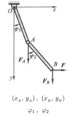
图中的 $\varphi_1, \varphi_2$ 就是广义坐标，经典的正交坐标 $(x_A, y_A), (x_B, y_B)$ 就可以用这两个广义坐标表示

\begin{cases} x_A = L_1 s\varphi_1 \\ y_A = L_1 c\varphi_1 \\ x_B = L_1 s\varphi_1 + L_2 s\varphi_2 \\ y_B = L_1 c\varphi_1 + L_2 c\varphi_2 \end{cases}

5.3.2 Lagrangian 方程#

设 $\mathcal{K}$ 为系统动能， $\mathcal{P}$ 为系统势能，定义 Lagrangian 函数为

\mathcal{L} = \mathcal{K} - \mathcal{P}

则有方程

\boxed{ \frac{\mathrm{d}}{\mathrm{d} t}(\frac{\partial L}{\partial \dot q_k}) - \frac{\partial L}{\partial q_k} = \tau_k, \quad k = 1, \dots, n }

其中 $\tau = \begin{bmatrix} \tau_1 \\ \vdots \\ \tau_n\end{bmatrix}$ 为非保守广义力， $q = \begin{bmatrix} q_1 \\ \vdots \\ q_n\end{bmatrix}$ 为广义坐标， $\tau_k$ 是与 $q_k$ 对应的非保守广义力。

平面2R的Lagrangian解法

解：

设广义坐标为两个关节变量 $\theta_1$ 和 $\theta_2$ ，则

\begin{cases} x_1 = L_1c\theta_1 \\ y_1 = L_1s\theta_1 \\ x_2 = L_1c\theta_1 + L_2c(\theta_1 + \theta_2) \\ y_2 = L_1s\theta_1 + L_2s(\theta_1 + \theta_2) \end{cases}

对时间求导 (在绝对框架中的表达，不需要考虑框架的变化项)，得到

\begin{cases} \dot x_1 = - L_1\dot\theta_1s\theta_1 \\ \dot y_1 = L_1\dot\theta_1c\theta_1 \\ \dot x_2 = - L_1\dot\theta_1s\theta_1 - L_2(\dot\theta_1 + \dot\theta_2)s(\theta_1 + \theta_2) \\ \dot y_2 = L_1\dot\theta_1c\theta_1 + L_2(\dot\theta_1 + \dot\theta_2)c(\theta_1 + \theta_2) \end{cases}

于是

\begin{aligned} v_1^\top v_1 &= \dot x_1^2 + \dot y_1^2 = L_1^2\dot\theta_1^2 \\ v_2^\top v_2 &= \dot x_2^2 + \dot y_2^2 = L_1^2\dot\theta_1^2 + L_2^2(\dot\theta_1 + \dot\theta_2)^2 + 2L_1L_2\dot\theta_1(\dot\theta_1 + \dot\theta_2)c\theta_2 \end{aligned}

由此可得动能、势能 (零势能点可以任意选取)、Lagrangian 函数分别为

\begin{aligned} \mathcal{K} &= \frac{1}{2}m_1v_1^\top v_1 + \frac{1}{2}m_2v_2^\top v_2 \\ &= \frac{1}{2}(m_1 + m_2) L_1^2 \dot\theta_1^2 + \frac{1}{2}m_2L_2^2(\dot\theta_1 + \dot\theta_2)^2 + m_2L_1L_2\dot\theta_1(\dot\theta_1 + \dot\theta_2)c\theta_2 \\ \\ \mathcal{P} &= m_1gy_1 + m_2gy_2 = m_1gL_1s\theta_1 + m_2g(L_1s\theta_1 + L_2 s(\theta_1 + \theta_2)) \\ \\ \mathcal{L} &= \mathcal{K} - \mathcal{P} \\ &= \frac{1}{2}(m_1 + m_2) L_1^2 \dot\theta_1^2 + \frac{1}{2}m_2L_2^2(\dot\theta_1 + \dot\theta_2)^2 + m_2L_1L_2\dot\theta_1(\dot\theta_1 + \dot\theta_2)c\theta_2 - m_1gL_1s\theta_1 - m_2g(L_1s\theta_1 + L_2 s(\theta_1 + \theta_2)) \end{aligned}

于是，分别求出

\begin{aligned} \frac{\partial \mathcal{L}}{\partial \dot\theta_1} &= (m_1 + m_2) L_1^2 \dot\theta_1 + m_2 L_2^2(\dot\theta_1 + \dot\theta_2) + m_2L_1L_2(\dot\theta_1 + \dot\theta_2)c\theta_2 + m_2L_1L_2\dot\theta_1c\theta_2 \\ \frac{\partial \mathcal{L}}{\partial \dot\theta_2} &= m_2L_2^2(\dot\theta_1 + \dot\theta_2) + m_2L_1 L_2\dot\theta_1 c\theta_2 \\ \frac{\partial L}{\partial \theta_1} &= -(m_1+m_2)gL_1c\theta_1 -m_2gL_2c(\theta_1 + \theta_2) \\ \frac{\partial L}{\partial \theta_2} &= -m_2L_1L_2\dot\theta_1(\dot\theta_1 + \dot\theta_2)s\theta_2 - m_2gL_2c(\theta_1 + \theta_2) \end{aligned}

接着计算

\begin{aligned} \frac{\mathrm{d}}{\mathrm{d} t}(\frac{\partial \mathcal{L}}{\partial \dot\theta_1}) &= m_1L_1^2\ddot\theta_1 + m_2L_1^2\ddot\theta_1 +m_2L_2^2\ddot\theta_1 + m_2L_2^2\ddot\theta_2 + 2m_2L_1L_2\ddot\theta_1c\theta_2 - 2m_2L_1L_2\dot\theta_1\dot\theta_2s\theta_2 + m_2L_1L_2\ddot\theta_2c\theta_2 - m_2L_1L_2\dot\theta_2^2s\theta_2 \\ \frac{\mathrm{d}}{\mathrm{d} t}(\frac{\partial \mathcal{L}}{\partial \dot\theta_2}) &= m_2L_2^2(\ddot\theta_1 + \ddot\theta_2) + m_2L_1L_2\ddot\theta_1c\theta_2 - m_2L_1L_2\dot\theta_1 \dot\theta_2 s\theta_2 \end{aligned}

于是得出动力学方程为

\begin{aligned} \tau_1 &= m_1L_1^2\ddot\theta_1 + m_2L_1^2\ddot\theta_1 +m_2L_2^2\ddot\theta_1 + m_2L_2^2\ddot\theta_2 + 2m_2L_1L_2\ddot\theta_1c\theta_2 - 2m_2L_1L_2\dot\theta_1\dot\theta_2s\theta_2 + m_2L_1L_2\ddot\theta_2c\theta_2 - m_2L_1L_2\dot\theta_2^2s\theta_2 + m_1gL_1c\theta_1 + m_2gL_1c\theta_1 + m_2gL_2c(\theta_1 + \theta_2) \\ \tau_2 &= m_2L_2^2\ddot\theta_1 + m_2L_2^2\ddot\theta_2 + m_2L_1L_2\ddot\theta_1c\theta_2 - m_2L_1L_2\dot\theta_1 \dot\theta_2 s\theta_2 + m_2L_1L_2\dot\theta_1(\dot\theta_1 + \dot\theta_2)s\theta_2 + m_2gL_2c(\theta_1 + \theta_2) \end{aligned}

化简得到

\boxed{ \begin{aligned} \tau_1 &= m_1L_1^2\ddot\theta_1 + m_2L_1^2\ddot\theta_1 +m_2L_2^2\ddot\theta_1 + m_2L_2^2\ddot\theta_2 + 2m_2L_1L_2\ddot\theta_1c\theta_2 - 2m_2L_1L_2\dot\theta_1\dot\theta_2s\theta_2 + m_2L_1L_2\ddot\theta_2c\theta_2 - m_2L_1L_2\dot\theta_2^2s\theta_2 + m_1gL_1c\theta_1 + m_2gL_1c\theta_1 + m_2gL_2c(\theta_1+\theta_2) \\ \tau_2 &= m_2L_2^2\ddot\theta_1 + m_2L_2^2\ddot\theta_2 + m_2L_1L_2\ddot\theta_1c\theta_2 + m_2L_1L_2\dot\theta_1^2s\theta_2 + m_2gL_2c(\theta_1 + \theta_2) \end{aligned} }

注意，动能项中含有一个 $\cos\theta_2$ ，千万不要因为忽略这一项的导数
计算不出错的最好办法是不要尝试去构造对称的式子，全部化成乘积相加的形式
通过观察各项下标的差异进行比对