

Definitions
The KL Divergence (KLD) is defined as
This is the standard form we typically use to measure how different two distributions are, which we call the forward KLD.
But there’s another way to look at it - what if we swap the roles of and ?
This gives us what we call the reverse KLD. While they might look similar, they behave quite differently in practice.
Experimental Results
Setup
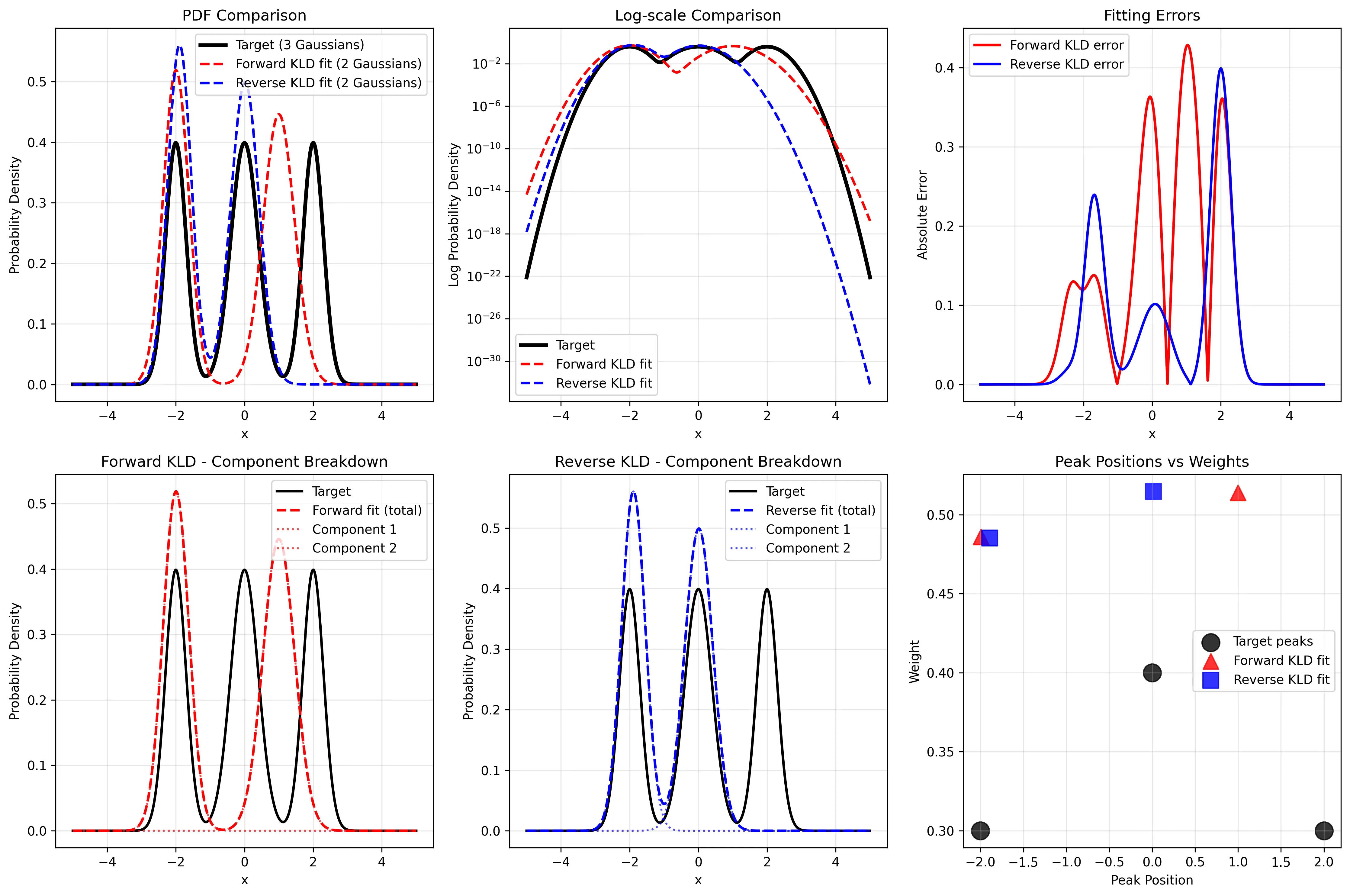
We fitted a 2-component Gaussian mixture to approximate a 3-component target distribution with peaks at positions [-2, 0, 2] and weights [0.3, 0.4, 0.3]. The KLD values were computed using Monte Carlo sampling with 20,000 samples to ensure numerical accuracy, rather than numerical integration which can suffer from discretization errors.
Observed Phenomena
Forward KLD Results:
- Means:
[-1.98, 1.97]- positioned near outer target modes - Standard deviations:
[0.41, 0.42]- wider to cover intermediate regions - Weights:
[0.52, 0.48]- balanced between components - Loss:
0.0012- very low
Reverse KLD Results:
- Means:
[-2.001, 0.010]- focused on the two strongest modes - Standard deviations:
[0.299, 0.418]- matching target component widths - Weights:
[0.426, 0.574]- proportional to target mode strengths - Loss:
0.3524- significantly higher
Key Behavioral Differences
Forward KLD creates a bimodal approximation that positions components to provide coverage across all target modes. The components are placed strategically to minimize the maximum approximation error across the entire distribution support.
Reverse KLD produces a selective approximation, focusing computational resources on the two most prominent modes (
x = -2andx = 0) while completely ignoring the rightmost peak atx = 2.Forward KLD uses broader components with balanced weights to ensure no region of significant target mass is left uncovered, while Reverse KLD uses component parameters that closely match the characteristics of the selected target modes.
Loss magnitude difference: Forward KLD achieves much lower loss values, indicating successful coverage of the target distribution, while Reverse KLD accepts higher loss in exchange for concentrated, high-fidelity approximation of selected modes.
Theoretical Explanation
The key to understanding these different behaviors lies in examining the mathematical forms and the role of the weighting function.
Mathematical Analysis
Let’s rewrite the two KLD formulations with emphasis on their weighting:
The crucial insight is that the first distribution in the KLD acts as the weighting function for the expectation.
Penalty Mechanisms
Forward KLD is weighted by :
- High penalty when is large but is small (since )
- Low penalty when is small, regardless of
- Consequence: must “cover” all regions where has significant mass
- Behavior: Zero-avoiding, mode-averaging
Reverse KLD is weighted by :
- High penalty when is large but is small (since )
- Low penalty when is small, regardless of
- Consequence: avoids placing mass where has little mass
- Behavior: Zero-forcing, mode-seeking
Asymmetric Risk
Consider what happens when versus :
| Scenario | Forward KLD | Reverse KLD |
|---|---|---|
| High penalty ( large) | Low penalty ( small) | |
| Low penalty ( small) | High penalty ( large) |
This asymmetry explains the observed behaviors:
- Forward KLD forces to “stretch” and cover all modes of
- Reverse KLD forces to “concentrate” and avoid low-probability regions of
Information-Theoretic Perspective
From an information theory standpoint:
- Forward KLD measures the extra bits needed when using code to compress data from
- Reverse KLD measures the extra bits needed when using code to compress data from
When optimizing :
- Forward KLD ensures can efficiently encode all data that might generate
- Reverse KLD ensures that data generates can be efficiently encoded by
This fundamental asymmetry drives the dramatically different optimization behaviors observed in our experiments.